Software
This section explains in detail the application side and describes the responsibility of each application in the Next Generation Smart Factory (NGSF) context.
The OPC UA applications control the system. These applications generate the control messages on the primary node and set the positions of the wheels on the servomotors.
Messaging between applications in this setup is based on OPC UA PubSub over Time Sensitive Networking (TSN), and the public open source Open62541 stack is used as a reference. Messaging drives the control of motors and measurements of key performance indicators (KPIs) at the same time.
The default use case is an open control loop, which means that measurements performed on the field controller FPGA node do not interfere with the next control message. Measurements are accumulated for one second on the secondary nodes and then sent as statistics to be shown on the dashboard.
Alternatively, NGSF provides an additional configuration that simulates a closed control loop by publishing a measurement for each control message that arrives on the end node and is collected by an additional application designed to run on the primary node.
The statistics can be visualized in the tsn_dashboard application, providing an overview of the quality of the system. For more details on this component, refer to the Dashboard section.
At a higher level, the industrial PC named Primary Node has the duty to produce control messages, which are transmitted to the Secondary Node and other Field Controllers FPGA nodes.
The workflow is:
Control messages are generated and published by the Primary Node as OPC UA PubSub TSN messages. All other nodes are subscribers of these messages.
Upon receiving a control message, an end node changes the driver state (if applicable) and performs measurements.
Measurements can be either immediately looped back and accumulated at the Primary Node, or can be accumulated at the end node.
Statistics for every end node are generated by the accumulator, end node or Primary Node, and sent every one second.
Dashboard receives the statistics and processes them according to its configuration.
The demonstration uses Intel® Edge Control for Industrial (ECI) to enable the TSN applications and allow time measurement in a real-time environment. ECI offers a real-time kernel and provides tools for clock synchronization and software drivers for the TSN network interfaces.
To keep clock synchronization, the Industrial PCs must run ptp4L and phc2sys. In the FPGA controllers selected for the NGSF setup, this functionality is enabled by default through the Edge PTP stack from TTTech*. For more information, refer to the TTTech DE board manual.
The applications that run on the Industrial PCs include the following:
Edge Control for Industrial package, which provides Real-Time Linux*,
ptp4L,phc2sys, and drivers.main_ctrl_apprunning on the Primary NodeC application producing control messages to the other nodes
main_meas_stats_apprunning on the Primary NodeC application receiving measurement messages from the end nodes and producing statistics as UDP messages. Its usage is optional depending on the use case that you want to simulate. By default, in an open loop setup, there is no need to execute this application.
sec_ctrl_apprunning on the Secondary NodeC application receiving control messages from the
main_ctrl_appand publishing measurements or statistics. By default, this application publishes statistics, that is, measurements are performed and a statistics message is sent at the end of one second.
tsn_dashboardis an HMI application running on either the Primary Node or an independent PC, depending on the setupReceives and displays the Statistics UDP messages from the end nodes or from
main_meas_stats_appand records them in a database.
On the FPGA side, there are two options: a setup with or without servomotors. As a common ground, the stack uses the TTTech TSN Switch IP modified for real-time applications. When controlling the servomotors, Drive on Chip (DoC) is added to the setup. For more details on how to generate this stack, contact Intel Programmable Solutions Group Support using the Contact us link on the webpage. TTTech Switch IP does not require manual execution of ptp4L or phc2sys, as mentioned, the stack executes them in the background.
The applications that run on the FPGAs include:
sec_fpga_ctrl_apprunning on an FPGA switched end node: Used to collect statistics on an FPGA that is not acting as a controller for the motorsmotor_fpga_ctrl_apprunning on the FPGA: Used to control the servomotor and perform measurements
These applications require configuration related to the setup they are running. For details, refer to Setup Two, where a setup with FPGAs is described.
A ngsf.json file is also used for the basic settings of the messaging protocol OPC UA Publisher subscriber. For more details, refer to OPC UA Messaging.
OPC UA Messaging
The core objective of NGSF is to demonstrate using deterministic network messages to coordinate mechanical action, by synchronizing two servomotors.
In the NGSF design, the Primary Node calculates the servomotor positions and publishes control messages. The control messages are consumed by the end nodes. On the field control devices, FPGAs, these messages are translated to drive impulses, thus setting the position of the servomotors. FPGAs perform the programming of the servomotors via the DoC component added to their software stack.
The control messaging protocol is OPC UA Publisher/Subscriber (PubSub) over TSN, which was chosen due to its popularity as an industrial communication protocol and its ease of deployment.
In the demo setup, the measurements show the robustness and determinism of the system. Therefore, each end node also does its own measurements that are either published immediately as Measurements messages or collectively published later as Statistics (the default setup is one second of measurements). Statistics messages carries the maximum, minimum, and average for every measured quantity.
Measurements messages, if generated, will be sent from all end nodes and collected on the primary node, which then summarizes and periodically sends out Statistics packets, using multicast UDP, to the dashboard.
The following figure shows the complete message flow, describing the node that is publishing and subscribing for a given message, and showing best effort and time critical messages.
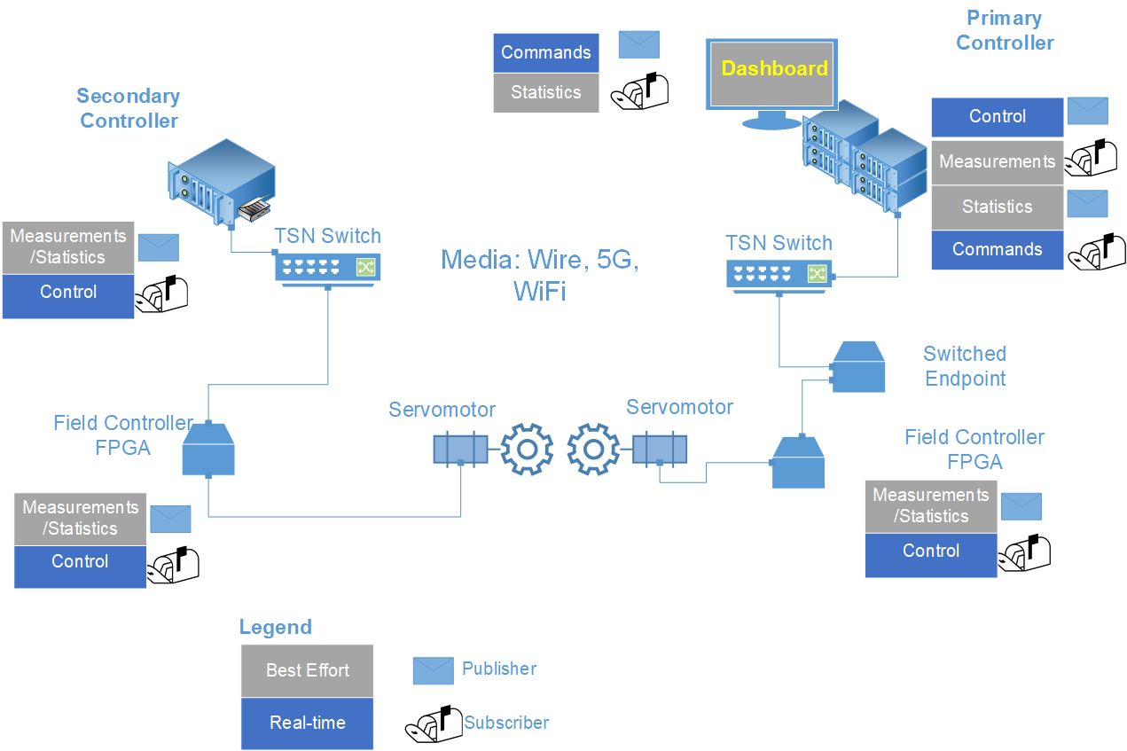
To summarize, the messages used in the setup are:
Control (Best Effort)
Measurements (Best Effort)
Statistics (Best Effort, not using OPC UA)
Command (Real-time, not implemented yet)
To enable communication and instantiate publishers and subscribers, you must define the following: a URL, a communication port, and certain OPC UA parameters including publisher ID, dataset writer ID, and writer group ID. This information is summarized in the configuration file for the setup. The name provided to this set of attributes in the demo is “Channel”, understood as a communication channel, as those values are used by the Publisher and Subscribers.
The following are the sample values used for the “Control” Channel:
"Control":{
        "url": "opc.eth://01-00-5E-7F-00-01:3.4",
        "pub_id": 2235,
        "dataset_writer_id": 62541,
        "writer_group_id": 101,
        "port": 62541
},
For a more detailed description of the application configuration, refer to :ref:`ngsf.json File`.
Message Architecture
Messages are designed to control the servomotors, and for providing ways for the end nodes to perform measurements relative to time and the current position or speed of the servomotor. The following figure lists the fields found in the messages (Control, Measurement, and Statistics messages).
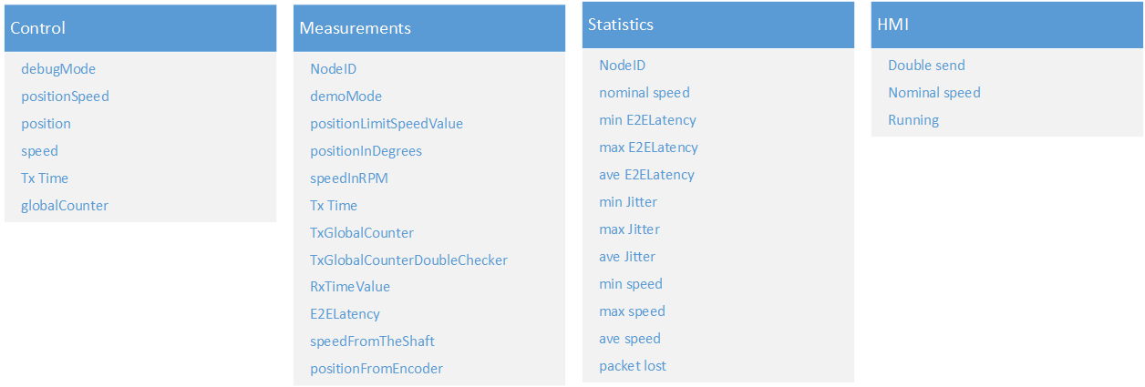
Control messages contain fields to drive the motor and fields to perform measurements. For example, Tx Time allows the measurement of the end-to-end latency and provides flexibility to the subscriber on how to use the messages.
The fields for control messages are:
debugMode: Determines if the motor will be in position or speed mode. By default, it is set to positionpositionSpeed: Defines the maximum permissible speed of the motor, which is set at 1300 rpm for safety reasonsposition: Calculated position to be programmed by the FPGA controllerspeed: Not usedTxTime: Value for calculating E2E latencyGlobal counter: Counter for calculating packet loss information
Every end node that subscribes to control messages may also publish a measurement message. Measurement messages have fields to allow FPGA and IPCs to perform measurements independent of the topology.
The fields for the Measurement message are:
Node ID: ID of the node, which must be unique in the networkDemo Mode: Returns the motor operational mode, either position or speedPosition Limit Speed Value: Returns the limit for the speed or position as read from the driverPosition in degrees: Current position measured by the driverSpeed in RPM: Nominal value of the speedTx Time: Time of the message that was sent from the controlTx Global Counter: Global counter as it is received from the control messageTx Global Counter Double checker: Returns the number of lost packages since the last correct package was deliveredRx Time: Time of receiving the packageE2E Latency: Difference between Rx and Tx (from control)Speed from the shaft: Speed as read from the servomotor shaftPosition from the encoder: Position as read from the encoder
The E2E latency, speed from the shaft, and TX Global Counter Double Checker fields are used to provide system information. Also, the position from the encoder can be used in combination with Rx time to get better information on the synchronization of the discs.
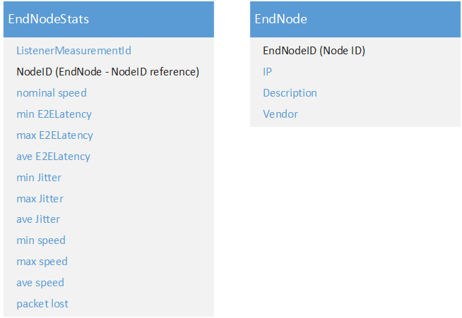
The Statistics message carries a summary of measurements for each end node acquired during the one second of measurements. The fields present on the Statistics message are:
Node ID: Same as in the Measurement message, that is, the ID of the node providing statistics(min, max, ave) RXCycle: Minimum, maximum, and average values for the inter-reception period(min, max, ave) PHC2Sys clock difference: Minimum, maximum, and average values for the difference between the system and the network (PHY) clock(min, max, ave) Sys clock read latency: Minimum, maximum, and average values for latency of reading the system clock(min, max, ave) PHY clock read latency: Minimum, maximum, and average values for latency of reading the network clock(min, max, ave) E2Edelay: Minimum, maximum, and average values for the end-to-end delay(min, max, ave) Jitter: Minimum, maximum, and average values for jitter(min, max, ave) Speed: Minimum, maximum, and average values for the speed from the shaft and is not applicable for all end nodesNominal position value: Vector of the positions of the wheels during last one secondPacket lost: Number of packages lost during last one second
OPC UA Configuration
This section describes the parameters required by OPC UA PubSub to establish a connection. For more information on the meaning of the parameters and their meanings for the OPC UA PubSub communication, refer to (OPC UA PubSub, 2021).
A publisher-subscriber (PubSub) communication requires the publishers and subscribers of a message to know the configuration or configuration parameters of each other, at least partially. This is addressed in the application configuration file called ngsf.json.
Time Measurements
This section describes the usage of messages to perform measurements.
The following figure shows the temporal relation between the Tx and Rx events as recorded and the end-to-end latency. In practical terms independent from the setup, the presented time measurement is an important measurement to be done.
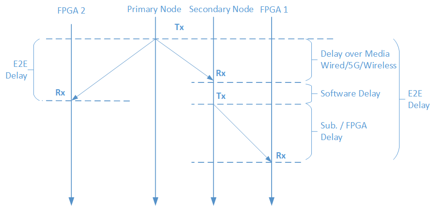
Note that for a meaningful measurement, the network clocks and the system clocks must be synchronized. As the synchronization of the network clocks and the system clocks happens independently in every node and are subject to drifts, it is important to evaluate measurements of the clock accuracy and the latencies.
Dashboard
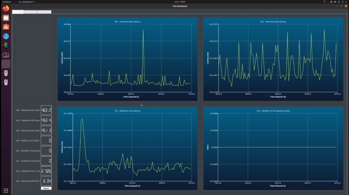
The dashboard application is a graphical user interface (GUI) for the NGSF setup, which receives, displays, and stores the Statistics messages. The dashboard has three tabs in order: Live Data, Long Term, and Preferences.
Live Data has four graphs and eight numbers that are updated as data arrives at the dashboard application.
Long Term has four graphs showing histograms and box plot graphs, which are updated by user interaction. The Long Term tab displays all measurements acquired from the start until the moment of the plot, thus providing additional insights over time. This tab offers a visualization tool, a time plot, a histogram, and a box plot, all in the same scale providing a comprehensive visualization of the measurements.
Preferences allows you to modify all elements. This tab displays the database for exporting, and provides means to describe end nodes. Exporting the database also provides the means to perform deeper analysis with the data via external tools, for instance, Python* scripting.
You can configure the graphs and numbers by right-clicking.
Note that to evaluate a complete configuration, data from all end nodes must have arrived at least once.
You can compare the position of the servomotors and calculate the sum of the error during the one-second period using the Live Data and Long Term displays. To do this, you must first add a comparison node using the Preferences tab, which creates a dedicated channel to identify the message arrival at the specified end nodes and then process them pairwise. Next, the values are calculated and displayed by the graphic elements. This feature will be extended in future versions of NGSF.
The following section describes the tabs in detail.
Live Data display
The Live Data display provides an overview of the current setup status with an interface to steer the servomotors. The following figure shows the Live Data display. The lower left pane is a numerical display for the most prominent numbers.
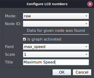
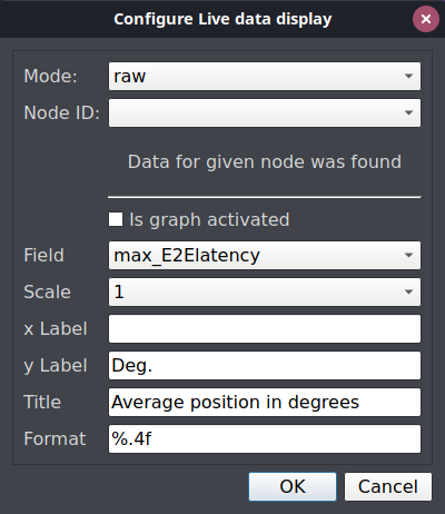
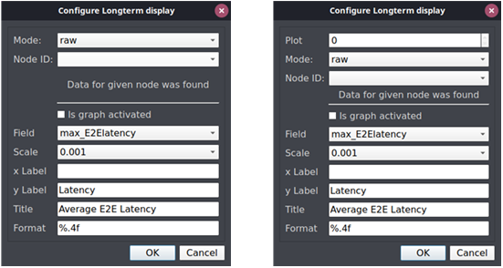
You can right-click the graphical elements to configure the Live Data displays or LCD numbers. The following figures show the dialogs for configuring LCD and Plot, respectively.
|
|
The fields to be configured are:
Mode: Raw or Comparison
NodeID: In Raw mode, this represents the end nodes in the setup that produce Statistics messages. In Comparison mode, this is the comparison ID node, artificially created when a comparison of two nodes is created.
Field: Selectable item, possible values are within the Statistics messages for the raw mode and among the comparison results for the comparison mode.
Scale: Multiplying factor for the value presented on the database.
X Label: Label to be used on X axis of the plot.
Y Label: Label to be used on Y axis of the plot.
Title: Title of the plot or LCD number.
Format: Format to be used on the X scale and %.4f stands for four precision digits.
On the Preferences tab, in the Live data section, enter or choose a value in the Seconds on graphs spin box to configure the number of points to be displayed on the live-data plot. After modifying that value, the number of seconds displayed on all live data graphs will change.
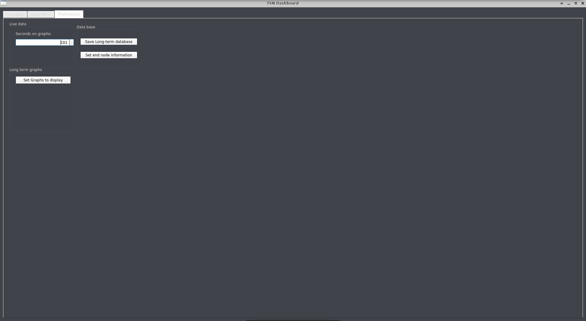
You can also configure the LCDs and Plots the Preferences tab. An additional field on the dialog indicates the index of the LCD number or the Plot for the Live display graphs.
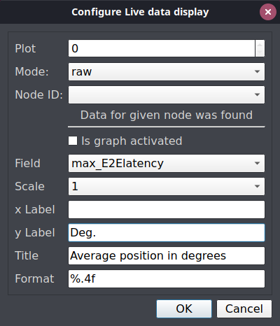
LCD numbers range from 0 to 7 from top to bottom and plots from 0 to 3 from top left to bottom right.
Database
The long-term display is driven by an SQLite database, which a simple interface for an application to use the data already received. The database is stored in a file, allowing another application to use the file for deeper analysis.
To describe the data, a relational scheme with four tables is used. There are two measurement tables: one for the raw statistics, named EndNodeStats and another called Comparison results. The end nodes producing the results are numbered with the ID numbers provided in the ngsf.json configuration file for the application and the numbers are kept in the EndNode table. The EndNodeIDs are related to the NodeID present in every entry of the EndNodeStats. The ComparisonNodes table have the fields ID1 and ID2 that are also EndNodeIDs, representing the nodes that are in a comparison item. By creating a new comparison node, a new CompID is created and every new measurement for this CompID is stored in the ComparisonResults.
Each new data entry on EndNodeStats receives a new key to make a new measurement unique. Note that no optimizations were done for the performance of the database. The goal is to keep the design simple and the use of queries straightforward to plot the data.
When the TSN_dashboard application starts, it backs up the old database file, if any, and creates a new one named longterm_tsn.db3. When the program terminates, this file can be copied or moved to any other location.
A simple query such as: SELECT * FROM endnodesstats WHERE EndNodeID == 0 retrieves all data available for the node 0 ordered by the ListenerMeasurementID, that is, chronologically ordered.
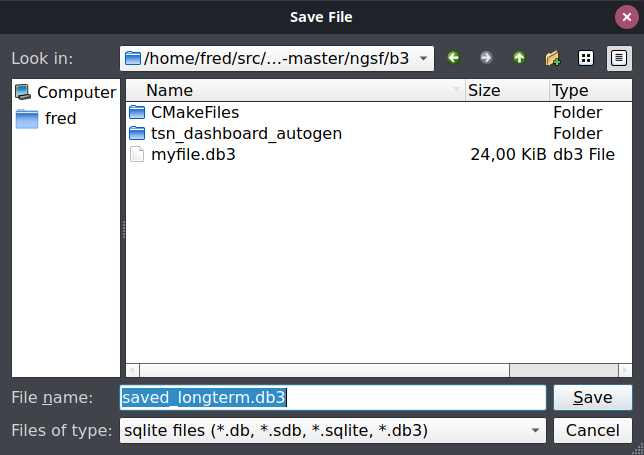
To export the database, go to the Preferences tab and click Save Long-term database from the Data base group. A dialog to set the directory and file name is displayed, as shown in the following figure.
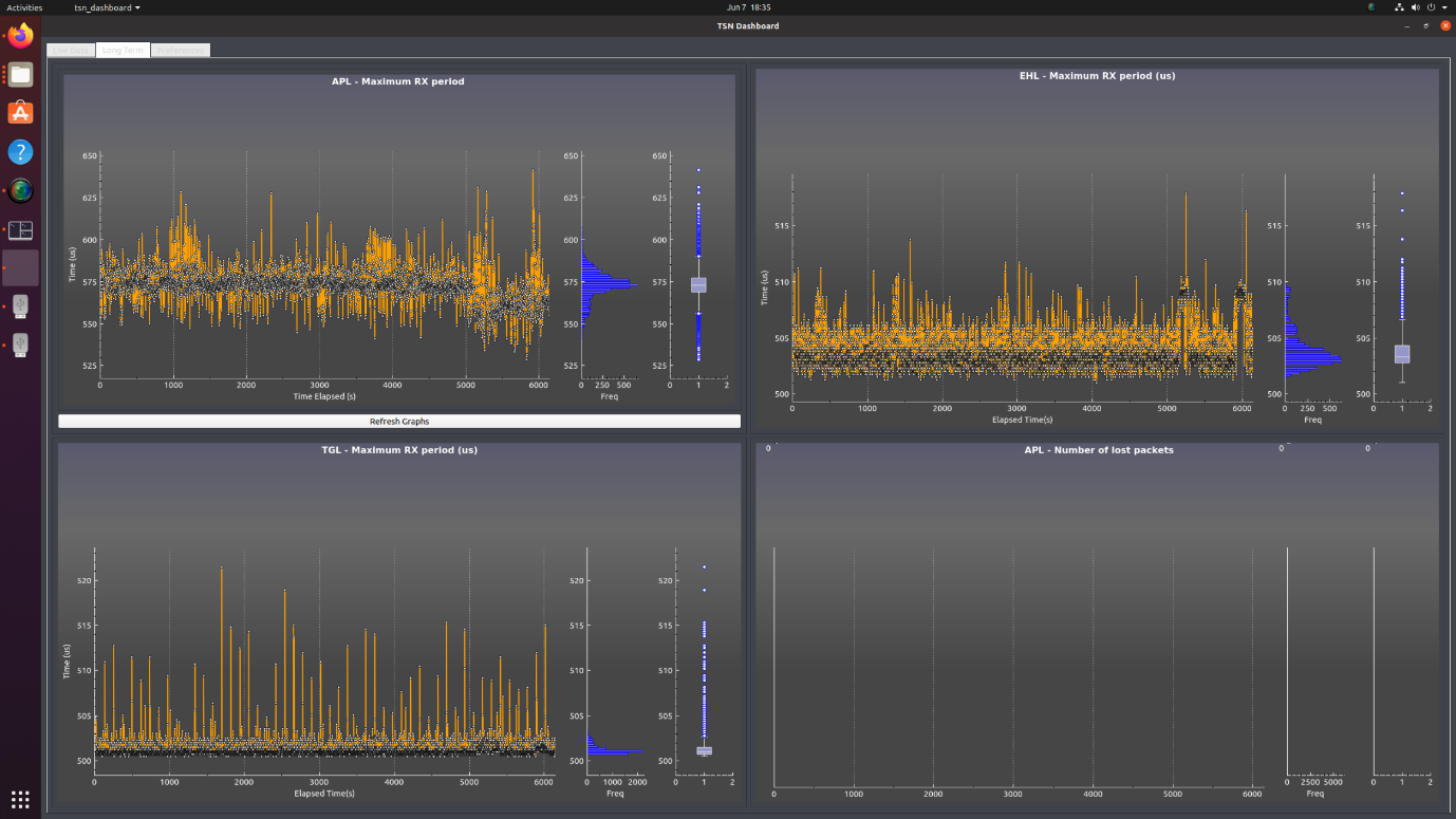
Long Term Display
The Long Term display provides an overview of the system over a longer time span, favoring unattended tests. Maximum and minimum delay and jitters, among other quantities, for any of the end nodes can be visualized, without the use of an external tool, at any time.
For an improved visualization, three kinds of plots are provided in the same scale:
Time plot, which provides an overview of time evolution and periodicity of values, and the possibility to visually correlate different measurements. For example, the end-to-end latency and clock synchronization.
The histogram shows more details of the distribution, but can hide outliers that are more clearly visible by the box plot. The following figure shows a Long-term display with the time, histogram, and box plot for three of the measurements done at the secondary node.
Long term graphs can display comparisons once they are added in the application. However, it is not possible to make any visual correlation from other measured quantities.
Long Term plots have the same fields as the Live Data plots and you can right-click the graph or use the button on the Preferences tab to configure. The following figures show both the plots.
Configuring Long Term graphs is similar to that of configuring Live data display. For more information, refer to Live Data display.
Preferences and settings
The Preferences tab provides an overview of the possible settings and additional interface for the database.
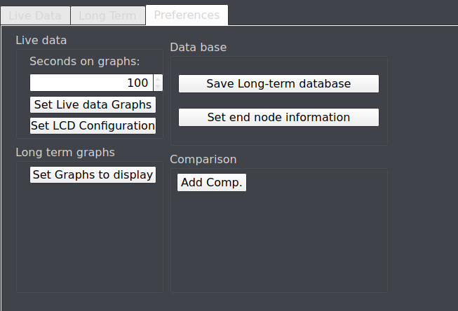
In the Live Data group, you can set the number of points on the live data plots, the data that each plot will display, and the values that the LCD numbers will show. For more details, refer to Live Data display.
In the Long Term graphs group, there is a single button to configure the Long term graphs. The fields are the same as those presented on the Live data graphs.
The Database group presents two buttons: one to save the database while running and another to set information for the end nodes.
All preferences are stored in an .ini file in the same directory where the tsn_dashboard binary runs. Every configuration setting is restored when the application is restarted. It is recommended that you do not edit the .ini file outside of the tsn_dashboard application.